Deep-learning models have achieved incredible breakthroughs on specialized tasks (e.g. image and text processing) but are not yet considered state-of-the-art on generic tabular data. For everyday generic classification and regression tasks, ensemble models based on decision trees, such as Random Forest and Gradient Boosted Trees, are still the go to workhorses (Grinsztajn et. al.).

Decision trees, however, suffer from the curse of dimensionality: the number of tree branches grows exponentially with the number of features, requiring exponentially large amount of training data (Bengio et. al.). This leads to oversized models with poor ability to generalize, especially when the available training data available is small relative to the number of features. Ensembling trees helps mitigate the negative effects of dimensionality, but it increases model complexity even further.

In this post we compare the performance of QCML against a variety of popular tree-based models (Random Forest, XGBoost, LightGBM and CatBoost) on high-dimensional tabular data. In contrast to trees, QCML learns a representation of the data into a small-dimensional compact space of quantum states, and it represents features as quantum measurements (Candelori et. al.). The number of parameters in a QCML model therefore scales linearly with the number of features, breaking the curse of dimensionality. This leads to a better ability to generalize, especially on smaller data sets with a large number of features.

Let's have a closer look.

Dataset creation

For this test we need to be able to generate families of data sets with an increasing number of features. An easy way to do this in Python is to use Scikit-learn's make_classification method

from sklearn.datasets import make_classification
from sklearn.model_selection import train_test_split

X,y = make_classification(n_samples=10000, 
                          n_features=1000, 
                          n_informative=1000, 
                          n_redundant=0, 
                          n_clusters_per_class=1,
                          class_sep=2,
                          n_classes=10,
                          random_state=0)

X_train, X_test, y_train, y_test = train_test_split(X,y, test_size=0.3, random_state=0)

This code creates a dataset X consisting of 10000 data points grouped in 10 clusters of equal size, each cluster being centered around the vertex of a 1000-dimensional hypercube. For each point in X, the array y contains the corresponding cluster, labeled with integers 0-9. We set the class_sep=2 parameter to ensure good separation between the clusters, so that the classification problem is not too difficult to learn.

The number of informative features n_informative denotes the dimension of the hypercube, and it is set to be equal to the number of total features. This ensures that the data set does not lie entirely on a lower-dimensional ambient space. For our test, it is essential to have control over the intrinsic dimension of the data.

Finally, we use scikit-learn's built-in train_test_split function to create a random 70/30 split of the data for training/testing, and measuring generalization accuracy.

Decision Trees

Let's see first how well a decision tree performs:

from sklearn.tree import DecisionTreeClassifier
from sklearn.metrics import accuracy_score

tree = DecisionTreeClassifier(random_state=0)
tree.fit(X_train, y_train)
y_pred = tree.predict(X_test)
acc = accuracy_score(y_true=y_test, y_pred=y_pred)
print(acc)
0.131

The 0.13 accuracy obtained by the decision tree is only marginally better than the 0.1 we would get from randomly guessing a label. We can examine the complexity of the tree structure by enumerating the number of leaves and the depth of the tree:

tree.get_n_leaves(), tree.get_depth()
(2361, 36)

Clearly this level of complexity is unnecessary for a data set consisting of only 10 well-separated clusters. The model is struggling to generalize.

We experimented with different regularization hyperparameters, setting the maximum depth of the tree and the minimum samples per leaf, but even with extensive tuning, the decision tree does not exceed 0.16 accuracy. Because every feature is informative, pruning the tree also hinders accuracy.

To better illustrate the curse of dimensionality, we can vary the number of features in the data set and plot the accuracy of the decision tree vs. the number of features:

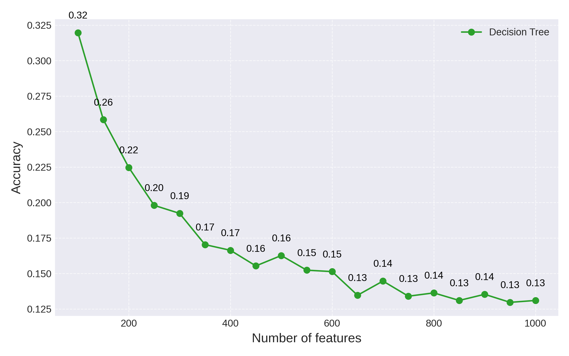
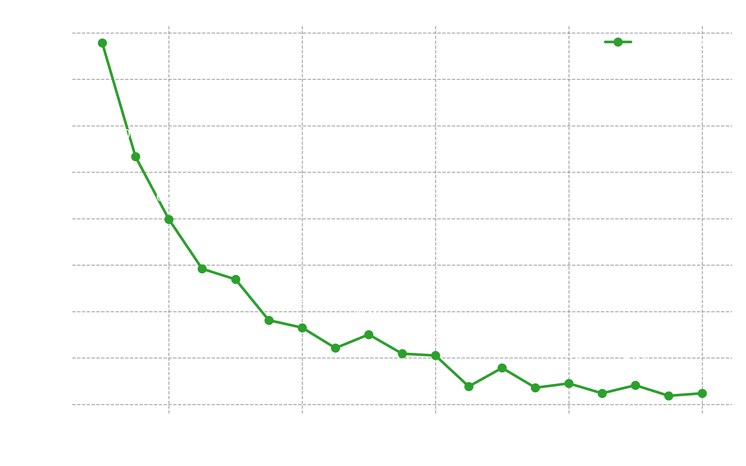
Fig 1: Decision tree accuracy as the number of features is increased

As expected, the performance of the decision tree degrades exponentially as the number of features is increased, approaching the baseline accuracy 0.1 of random guessing.

Random Forests

Decision trees are seldom used in isolation. The most common practice is to ensemble trees together into random forests. Ensembling hundreds or thousands of decision trees helps mitigate the negative effects of dimensionality (Bengio et. al. section 4.2) and leads to better generalization accuracy. However, as we show next, ensembling has diminishing returns as the trees approach baseline random accuracy.

We can test random forests on our 1000-dimensional dataset X by using the default RandomForestClassifier provided by scikit-learn, which ensembles 100 trees:

from sklearn.ensemble import RandomForestClassifier

rf = RandomForestClassifier(random_state=0, n_jobs=-1)
rf.fit(X_train, y_train)
y_pred = rf.predict(X_test)
acc = accuracy_score(y_true=y_test, y_pred=y_pred)
print(acc)
0.274

and similarly we can plot the accuracy on the test set as the number of features is increased:

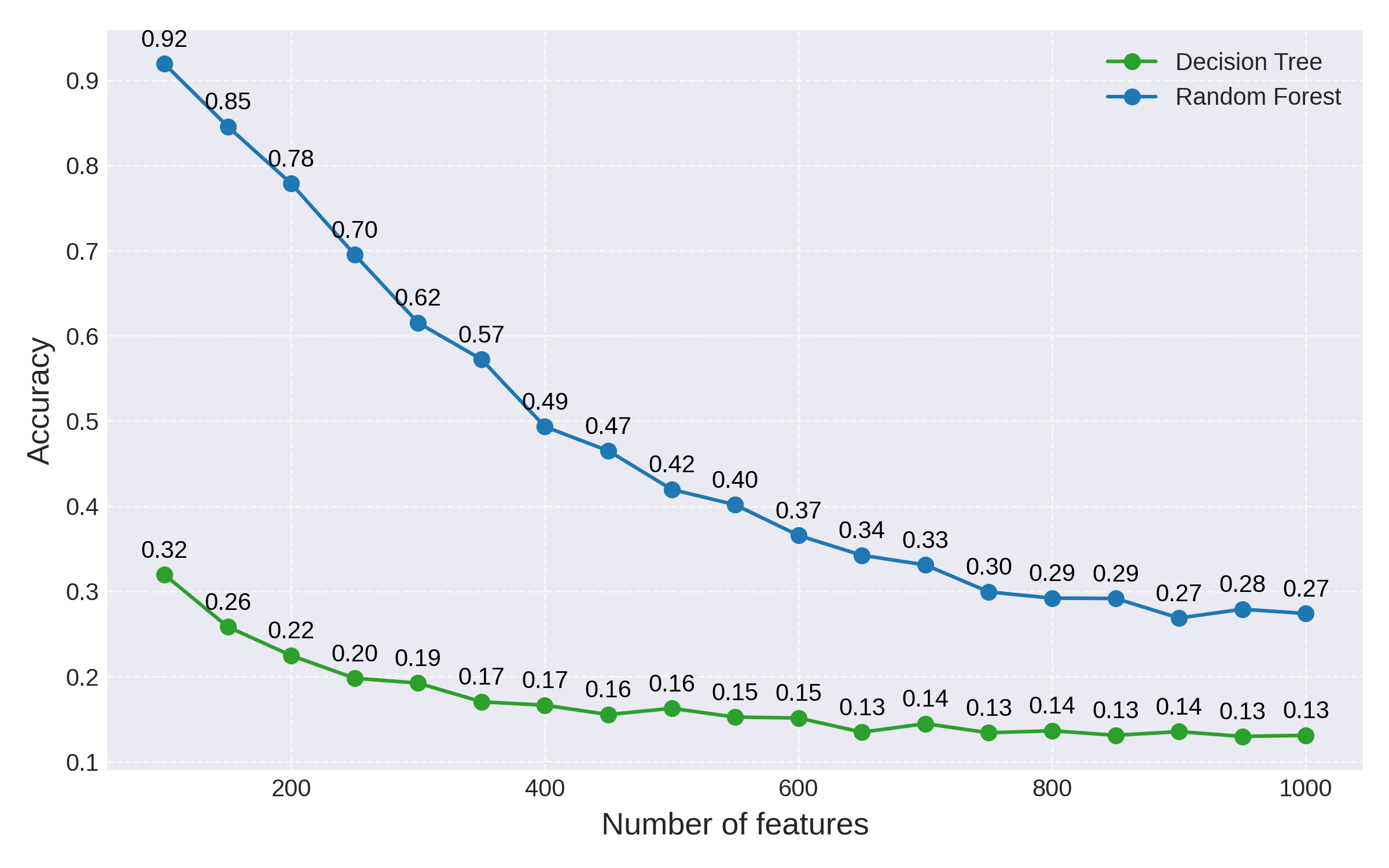
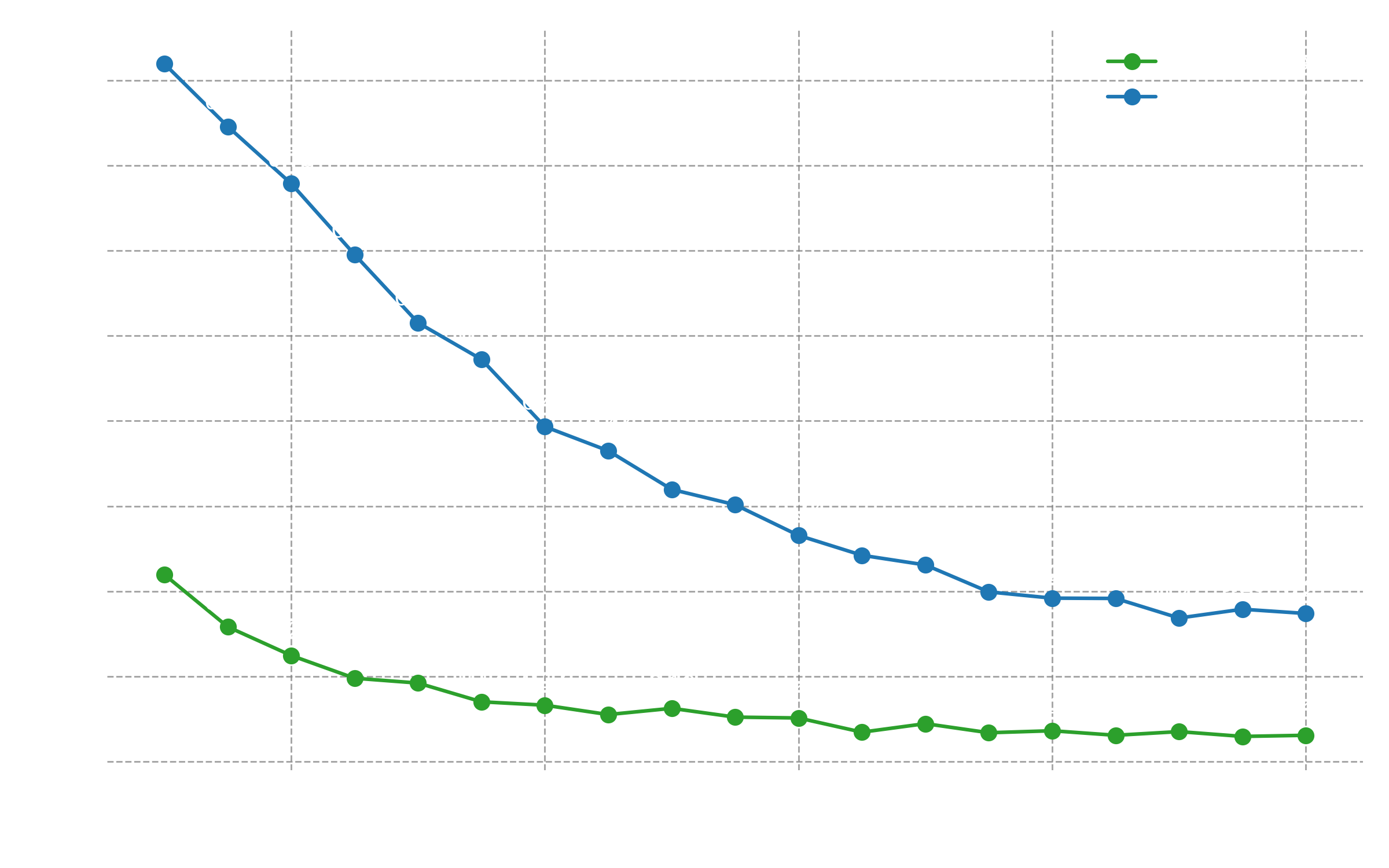
Fig 2: Accuracy comparison between a decision tree and a random forest

While ensembling leads to a dramatic performance improvement at first, this effect fades away as the number of features is increased: random forests clearly still suffer from the curse of dimensionality.

Increasing the number of trees in the forest will improve performance in this example, but it bogs down the model both in terms of running time and memory usage. As the number of features is increased even further beyond the 1000 range, this approach to breaking the curse of dimensionality becomes unfeasible.

QCML

Let's now compare performance with QCML. We can wrap a QCML model in a scikit-learn API (click here to request API access) and test it first on the original 1000-dimensional data set.

To keep the comparison level with other methods, we use default QCML hyperparameters: N=8 for Hilbert space dimension, 1000 training epochs and 0.1 learning rate.

qcml = QCMLClassifier(random_state=0)
qcml.fit(X_train, y_train)
y_pred = qcml.predict(X_test)
acc = accuracy_score(y_true=y_test, y_pred=y_pred)
print(acc)
0.862

Not only is the accuracy of QCML much higher than that of random forest for this particular 1000-dimensional example, the performance gap is also consistent across a range of features, as shown by the plot below:

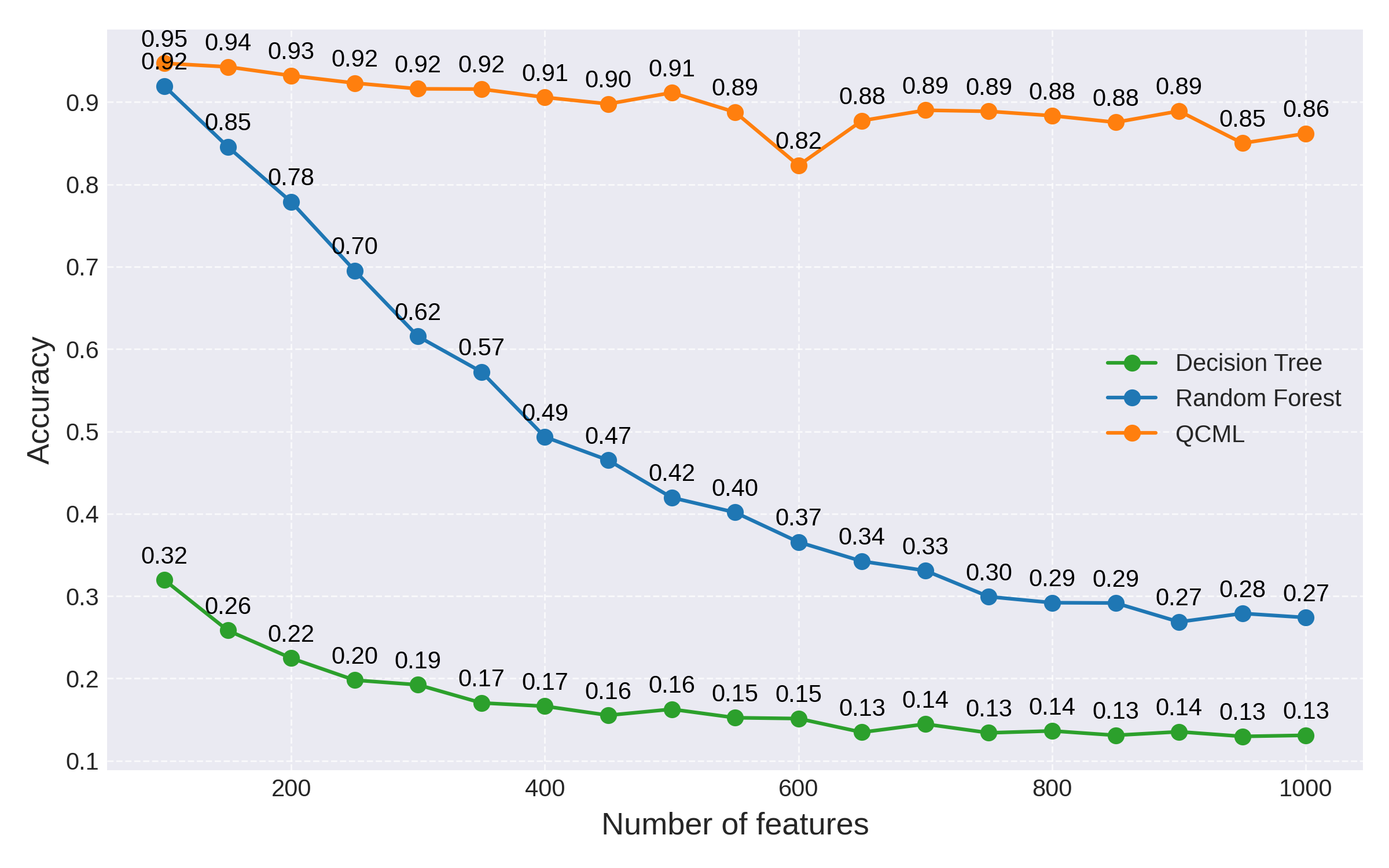
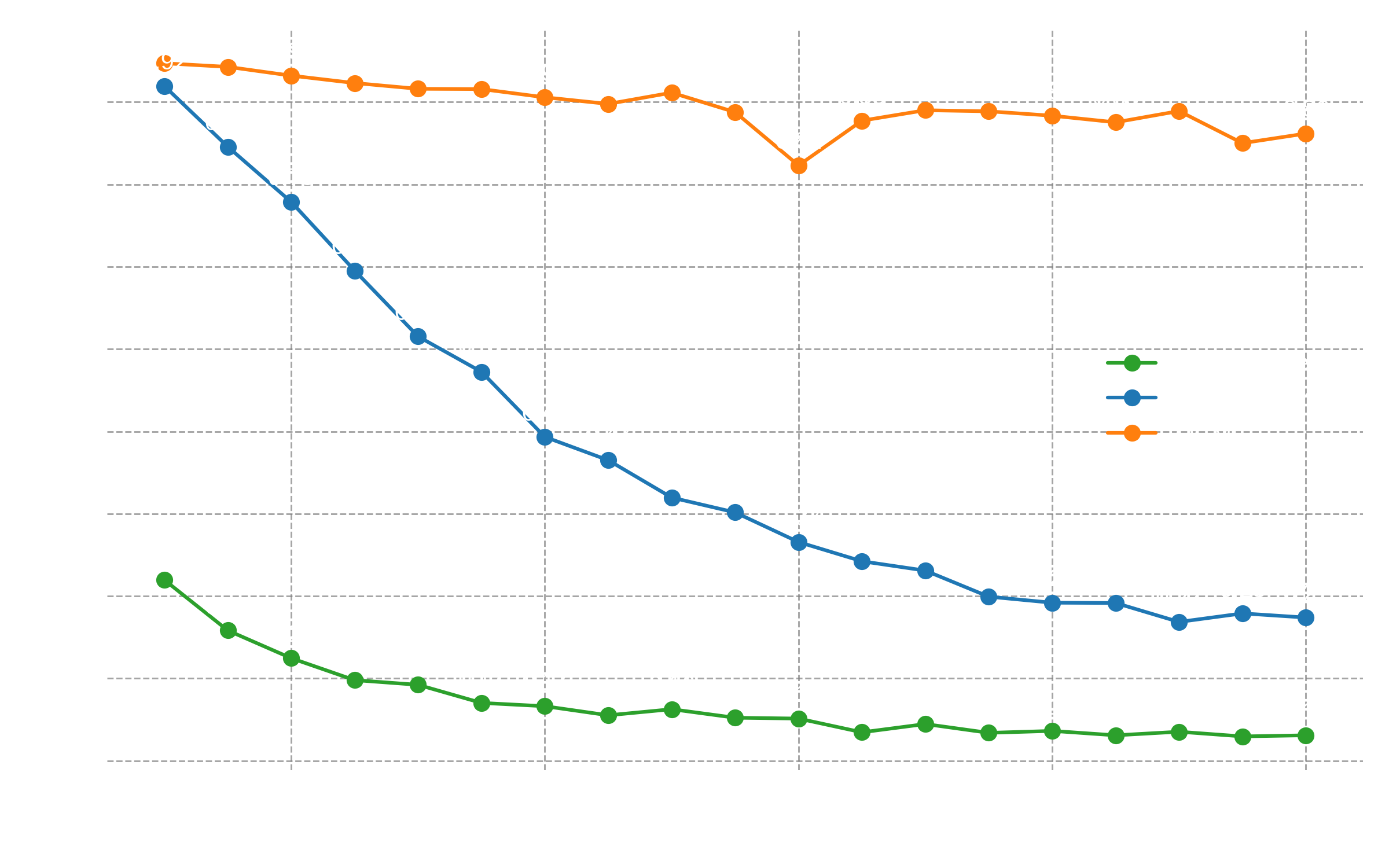
Fig 3: QCML accuracy remains high compared to Random Forest as the number of features is increased

While QCML is also affected negatively by the increased dimensionality, the degradation in generalization accuracy is only linear as opposed to an exponential in the case of random forest. Recall that the number of parameters scales linearly with the number of features for QCML, while it grows exponentially for random forest.

Increasing the size of the training set

We saw how the curse of dimensionality causes an exponential explosion in the size of a decision tree (or random forest), leading to worsening performance as the number of features increases and the training size remains constant. This is because larger models require larger training sets to generalize well.

For our original 1000-dimensional data set, we can test how many training data points we would need to add in order for a random forest model to match the accuracy of QCML:

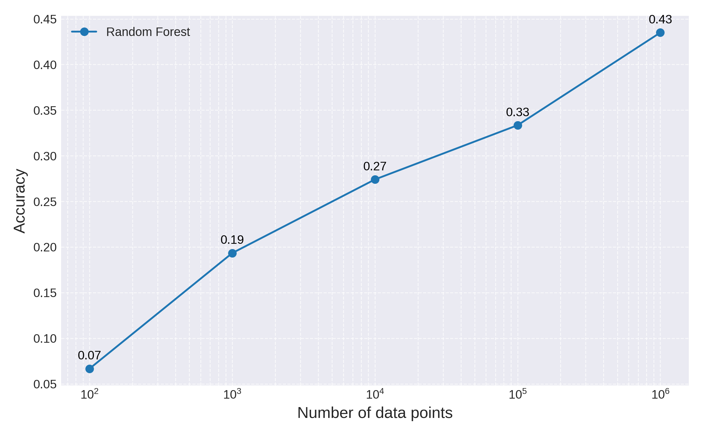
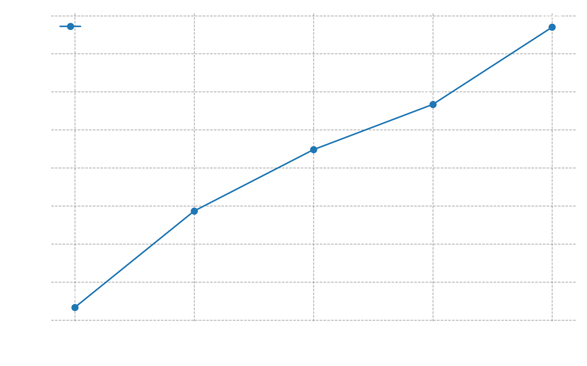
Fig 4: Random Forest accuracy as a function of training set size. Note the logarithmic scale for the x-axis

We can see a clear performance increase for Random Forest with larger training data. However, from the chart it is clear that this improvement is only logarithmic in the number of points. By a simple linear extrapolation we estimate that it would take random forest billions of training data points to match the accuracy of a QCML model trained on a few thousand points.

Gradient Boosted Trees

Next, we test three popular implementations of Gradient Boosted Trees (GBTs), which are also considered state-of-the-art on tabular data: XGBoost, LightGBM and CatBoost. These are more advanced ensembles of decision trees, where each tree is trained on the errors of the preceding one. Each implementation is optimized in different ways, and all three strive to provide optimal default hyperparameters. They all provide scikit-learn APIs, with Python code implementations very similar to the one for Random Forest provided above.

GBTs perform much better than Random Forest on our test. To really see a decline in performance got GBTs we push our test to 20000 features. Because of the higher dimensionality, we also increase the size of the data set to 50000 points, in order to facilitate training.

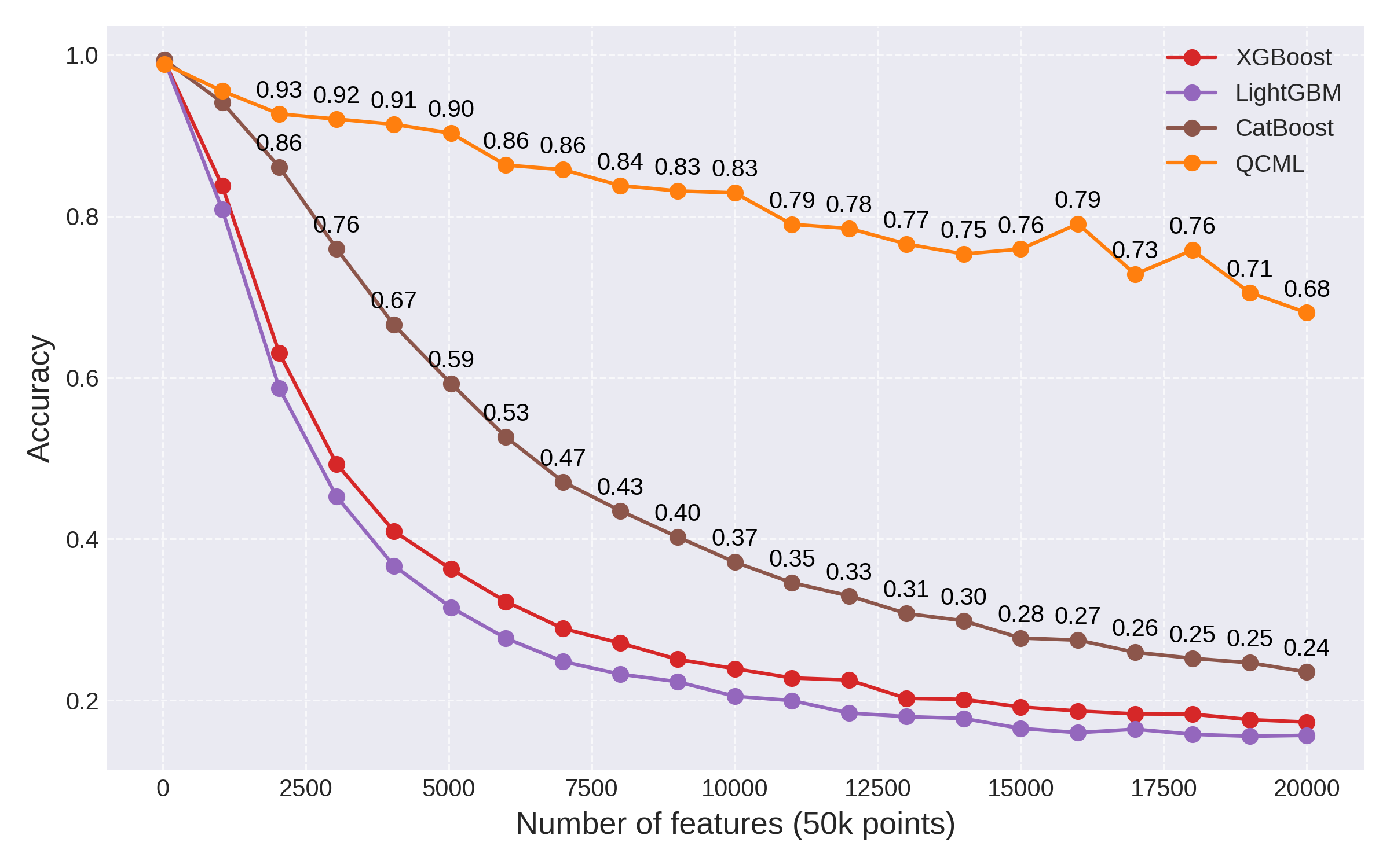
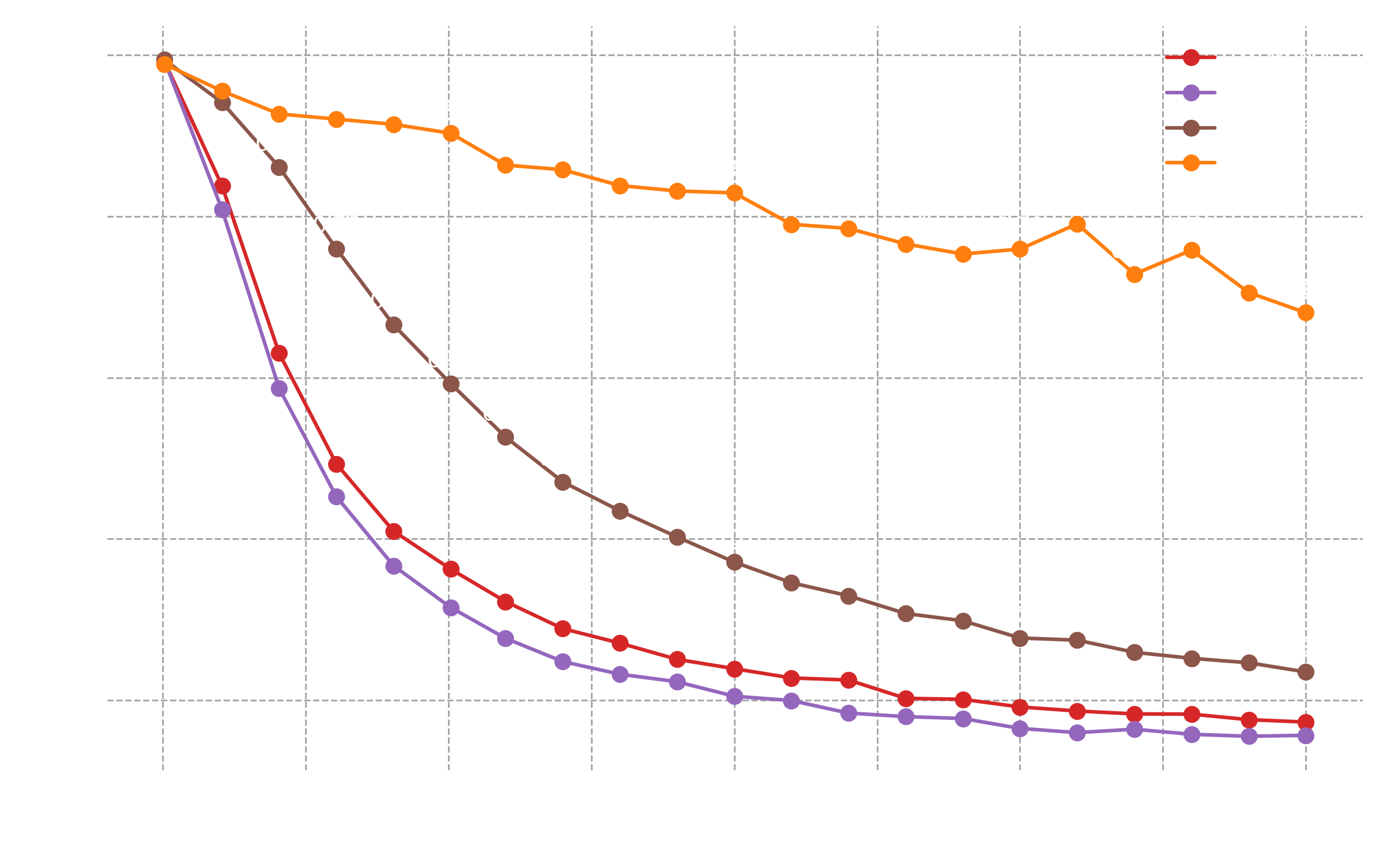
Fig 5: Comparison of different GBTs vs. QCML.

In the end, while GBTs do a pretty good job mitigating the curse of dimensionality, they are still subject to an exponential degradation of performance as the number of features is increased. By comparison, we see again that QCML's performance only degrades linearly. These fundamentally different scaling laws result in dramatic performance differences: at 20000 features, the best performing GBT (CatBoost) achieves an accuracy on the test set of 0.24, compared to the 0.68 accuracy clocked in by QCML.

Finally, we compare the performance of all three GBT models with respect to training set size. We ran this test with 5000 features and compared to QCML:

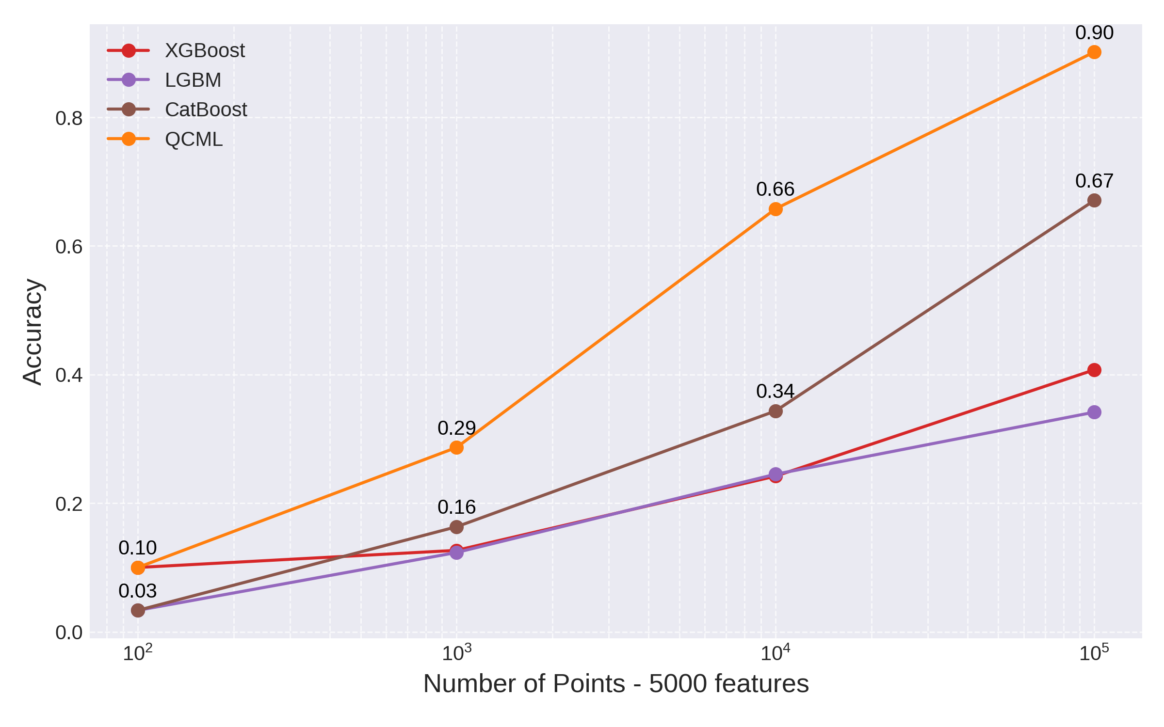
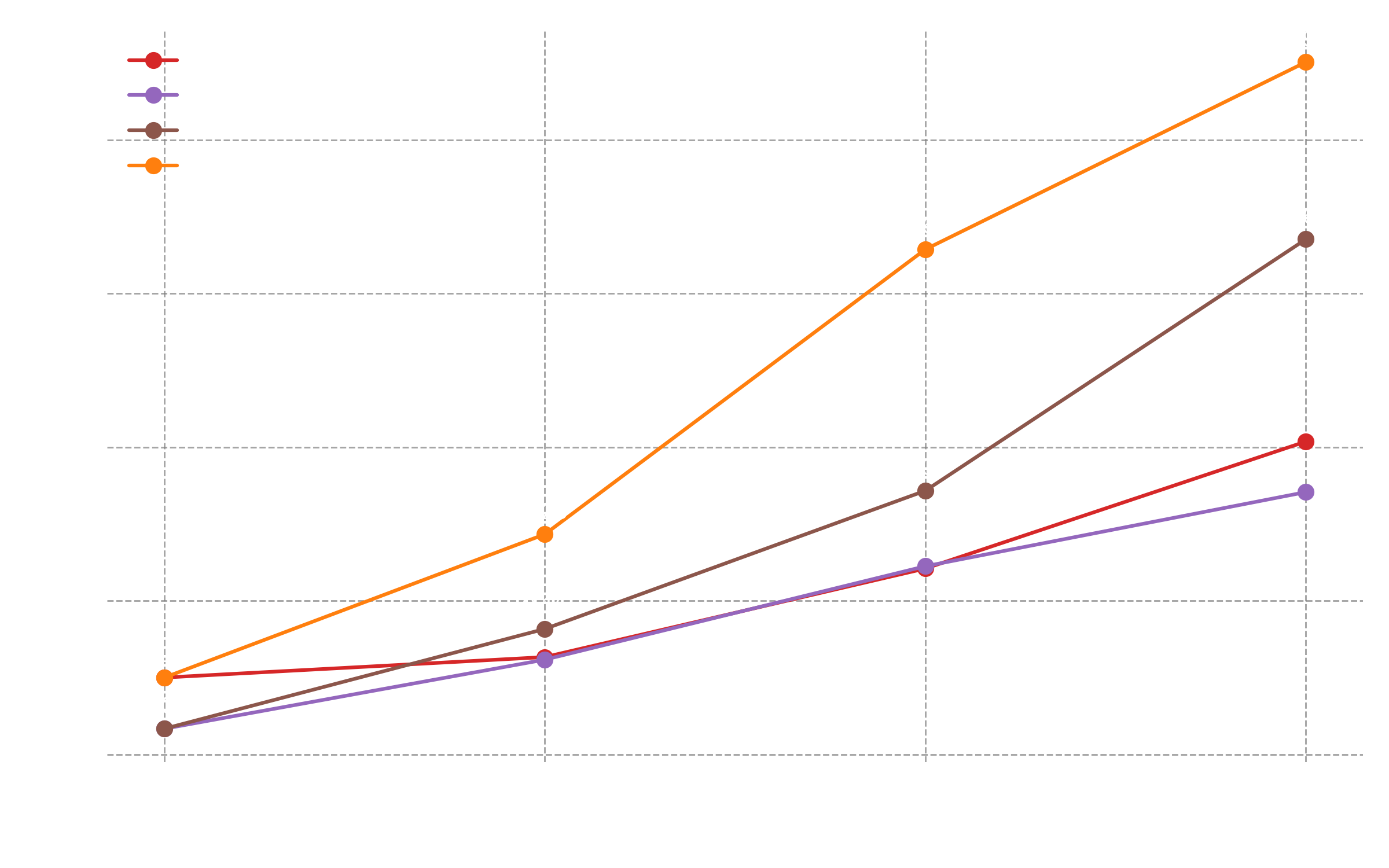
Fig 6: GBTs vs QCML accuracy as function of training set size with 5000 features

Clearly GBTs again offer increased performance compared to Random Forest and suffer less from the curse of dimensionality. However, even state-of-the-art GBTs implementation will require training sets of much larger size to achieve the same accuracy as QCML.

Conclusion

In this post we showed:

• All tree-based models (including Random Forests and GBTs) suffer from the curse of dimensionality on tabular data and exhibit performance degradation as the number of data features is increased.

• In contrast, QCML maintains higher levels of accuracy for high-dimensional data with fewer training samples.

These tests demonstrate that QCML outperforms state-of-the-art methods on high-dimensional tabular data, especially when the number of training samples is low compared to the number of features.